rsEGFP2 WT Switching QY

ON->OFF

Load Experimental Switching Data

We begin by importing the required library and loading the actinometry measurement data from a CSV file. The dataset is stored in exp_data for further analysis

import pandas as pd

exp_data = pd.read_csv("DATA/prot1 ON2OFF.csv")

exp_data

	timestamp	cycle	type	186.85486	187.31995223015844	187.78500323297956	188.250012996982	188.71498151068454	189.17990876260572	189.64479474126426	...	1032.9632529736894	1033.3204920667242	1033.6776665334785	1034.034776362471	1034.3918215422202	1034.7488020612445	1035.1057179080635	1035.4625690711953	1035.8193555391586	1036.176077300472
0	2025-04-04 13:05:43.323760	1	zero	16.990556	24978.543889	59.831028	47.330833	62.015528	71.481694	76.942944	...	470.274306	455.953694	458.259556	465.662583	459.958611	461.657667	467.847083	466.512111	466.512111	466.512111
1	2025-04-04 13:06:24.439856	1	on	16.990556	24978.543889	60.195111	42.233667	55.097944	67.234056	57.525167	...	457.774111	464.084889	463.114000	457.288667	441.511722	455.346889	469.182056	456.560500	456.560500	456.560500
2	2025-04-04 13:06:25.472725	1	on	16.990556	24978.543889	57.174568	48.544444	41.802160	43.150617	67.692531	...	453.081481	459.554074	460.632840	454.429938	472.229568	473.038642	461.981296	435.821235	435.821235	435.821235
3	2025-04-04 13:06:26.506516	1	on	16.990556	24978.543889	74.030278	60.437833	58.981500	54.369778	53.641611	...	462.871278	474.036500	470.881111	459.230444	455.346889	477.434611	456.075056	451.463333	451.463333	451.463333
4	2025-04-04 13:06:27.537642	1	on	16.990556	24978.543889	55.826111	47.195988	54.207963	80.907407	69.850062	...	471.690185	486.523210	459.823765	473.847716	457.126852	462.520679	440.945370	446.878580	446.878580	446.878580
...	...	...	...	...	...	...	...	...	...	...	...	...	...	...	...	...	...	...	...	...	...
386	2025-04-04 13:13:02.957585	1	on	16.990556	24978.543889	34.250802	37.756790	59.601790	63.916852	55.826111	...	435.281852	464.138827	449.575494	446.878580	447.957346	459.554074	450.384568	449.845185	449.845185	449.845185
387	2025-04-04 13:13:03.987853	1	on	16.990556	24978.543889	58.792716	15.372407	35.599259	54.747346	83.604321	...	463.599444	464.138827	464.138827	454.969321	460.363148	433.124321	450.923951	447.417963	447.417963	447.417963
388	2025-04-04 13:13:05.020339	1	on	16.990556	24978.543889	30.475123	42.880926	57.983642	69.040988	55.017037	...	471.150802	478.432469	456.048086	444.990741	465.217593	461.172222	452.002716	445.260432	445.260432	445.260432
389	2025-04-04 13:13:06.054197	1	on	16.990556	24978.543889	53.129198	22.923765	36.678025	38.835556	69.580370	...	438.248457	441.754444	446.339198	457.396543	455.239012	449.305802	435.281852	457.935926	457.935926	457.935926
390	2025-04-04 13:13:19.090390	1	static	16.990556	24978.543889	44.175444	36.772417	47.330833	41.505500	62.015528	...	439.812667	440.176750	464.813056	451.584694	446.851611	466.269389	448.672028	451.706056	451.706056	451.706056

391 rows × 2051 columns

Preprocess Spectral Data and Compute Absorbance

We now prepare the spectral intensity data for analysis. The dataset contains different types of measurements:

• “zero”: baseline measurements,

• “static”: background noise or dark reference,

• Other types: actual actinometry measurements over time.

We extract these components, convert timestamps, and compute the absorbance spectrum using the formula:

$$A(\lambda) = -\log_{10} \left( \frac{I(\lambda) - I_{\text{static}}(\lambda)}{I_{\text{zero}}(\lambda) - I_{\text{static}}(\lambda)} \right)$$

This normalization corrects for both dark current and reference intensity variations.

import numpy as np

intensities=np.array(exp_data[(exp_data["type"] != "zero") & (exp_data["type"] != "static")].iloc[:, 3:], dtype=np.float64)
static=np.array(exp_data[(exp_data["type"]== "static")].iloc[:, 3:], dtype=np.float64)[0]
zero=np.array(exp_data[(exp_data["type"]== "zero")].iloc[:, 3:], dtype=np.float64)[0]
wavelengths = np.array(exp_data.columns[3:], dtype=np.float64)
timestamps = pd.to_datetime(exp_data["timestamp"][(exp_data["type"] != "zero") & (exp_data["type"] != "static")]) # Convert timestamp strings to datetime objects
timestamps = np.array((timestamps - timestamps.iloc[0]).dt.total_seconds()) # Convert to seconds since the first timestamp

def compute_absorbance(intensities: np.ndarray, static: np.ndarray, zero: np.ndarray) -> np.ndarray:
    EPS = 1e-12
    num = intensities - static
    den = np.maximum(zero - static, EPS)  # Éviter division par zéro
    absorbance = -np.log10(np.maximum(num / den, EPS))  # Éviter log(0) ou log(négatif)
    return absorbance

absorbance = compute_absorbance(intensities, static, zero)

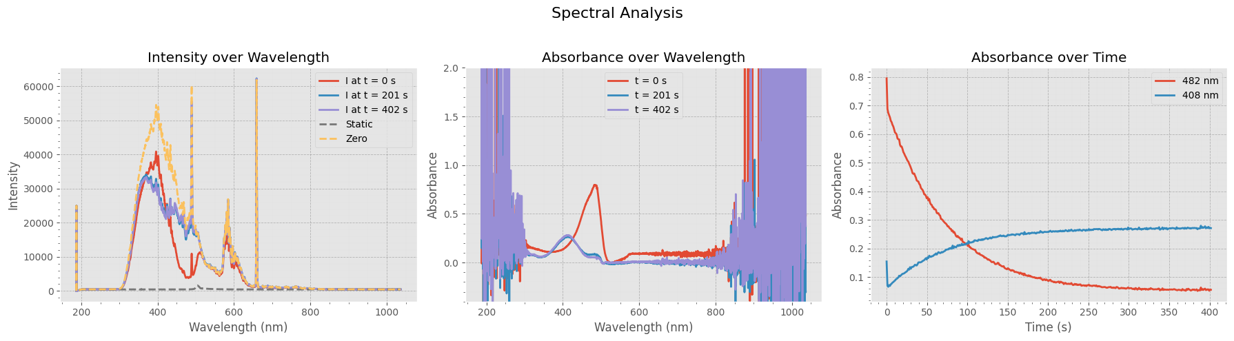
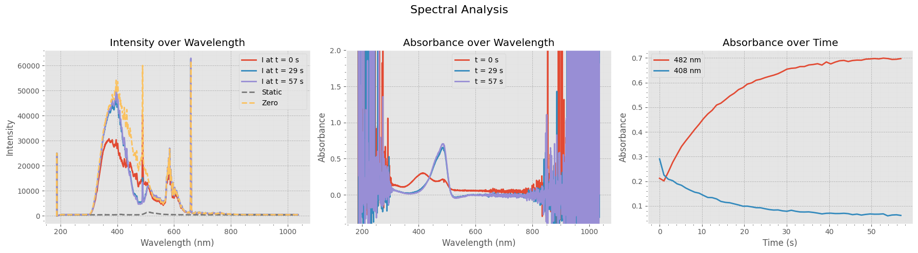
Visualizing Spectral Intensity and Absorbance

This figure provides a comprehensive view of the switching data:

1. Left Panel: Raw intensity spectra at three time points, along with the static and zero references.

2. Middle Panel: Corresponding absorbance spectra at the same time points, showing how absorption evolves over time.

3. Right Panel: Absorbance at two key wavelengths (482 nm and 408 nm) plotted as a function of time, highlighting dynamic changes in the sample.

These plots help assess the stability and dynamics of the measured signals and the quality of the zero/static references.

Show code cell source Hide code cell source

import matplotlib.pyplot as plt
import matplotlib.cm as cm
# Set global style
plt.style.use("ggplot")  # Clean style

fig, axs = plt.subplots(1, 3, figsize=(18, 5))
fig.suptitle("Spectral Analysis", fontsize=16)

# --- Intensity Plot ---
axs[0].plot(wavelengths, intensities[0, :], label=f"I at t = {timestamps[0]:.0f} s", linewidth=2)
axs[0].plot(wavelengths, intensities[len(intensities)//2, :], label=f"I at t = {timestamps[len(intensities)//2]:.0f} s", linewidth=2)
axs[0].plot(wavelengths, intensities[-1, :], label=f"I at t = {timestamps[-1]:.0f} s", linewidth=2)
axs[0].plot(wavelengths, static, '--', label="Static", linewidth=2)
axs[0].plot(wavelengths, zero, '--', label="Zero", linewidth=2)
axs[0].set_title("Intensity over Wavelength")
axs[0].set_xlabel("Wavelength (nm)")
axs[0].set_ylabel("Intensity")
axs[0].legend()
axs[0].grid(True, which='major', linestyle='--', linewidth=0.6, color='gray', alpha=0.5, zorder=0)
axs[0].minorticks_on()
axs[0].grid(True, which='minor', linestyle=':', linewidth=0.3, color='lightgray', alpha=0.4, zorder=0)
# --- Absorbance Plot ---
axs[1].plot(wavelengths, absorbance[0, :], label=f"t = {timestamps[0]:.0f} s", linewidth=2)
axs[1].plot(wavelengths, absorbance[len(absorbance)//2, :], label=f"t = {timestamps[len(absorbance)//2]:.0f} s", linewidth=2)
axs[1].plot(wavelengths, absorbance[-1, :], label=f"t = {timestamps[-1]:.0f} s", linewidth=2)
axs[1].set_title("Absorbance over Wavelength")
axs[1].set_xlabel("Wavelength (nm)")
axs[1].set_ylabel("Absorbance")
axs[1].set_ylim(-0.4, 2)
axs[1].legend()
axs[1].grid(True, which='major', linestyle='--', linewidth=0.6, color='gray', alpha=0.5, zorder=0)
axs[1].minorticks_on()
axs[1].grid(True, which='minor', linestyle=':', linewidth=0.3, color='lightgray', alpha=0.4, zorder=0)
# --- Absorbance vs Time Plot ---
WL = [482, 408]
idxs = [np.argmin(np.abs(wavelengths - wl)) for wl in WL]

for i, idx in enumerate(idxs):
    axs[2].plot(timestamps, absorbance[:, idx], label=f"{wavelengths[idx]:.0f} nm", linewidth=2)

axs[2].set_title("Absorbance over Time")
axs[2].set_xlabel("Time (s)")
axs[2].set_ylabel("Absorbance")
axs[2].legend()
axs[2].grid(True, which='major', linestyle='--', linewidth=0.6, color='gray', alpha=0.5, zorder=0)
axs[2].minorticks_on()
axs[2].grid(True, which='minor', linestyle=':', linewidth=0.3, color='lightgray', alpha=0.4, zorder=0)
plt.tight_layout(rect=[0, 0, 1, 0.95])
plt.show()

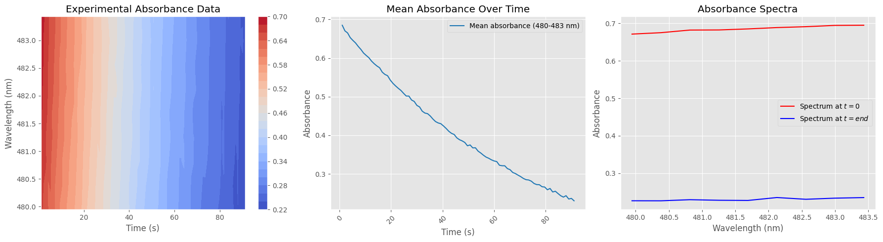
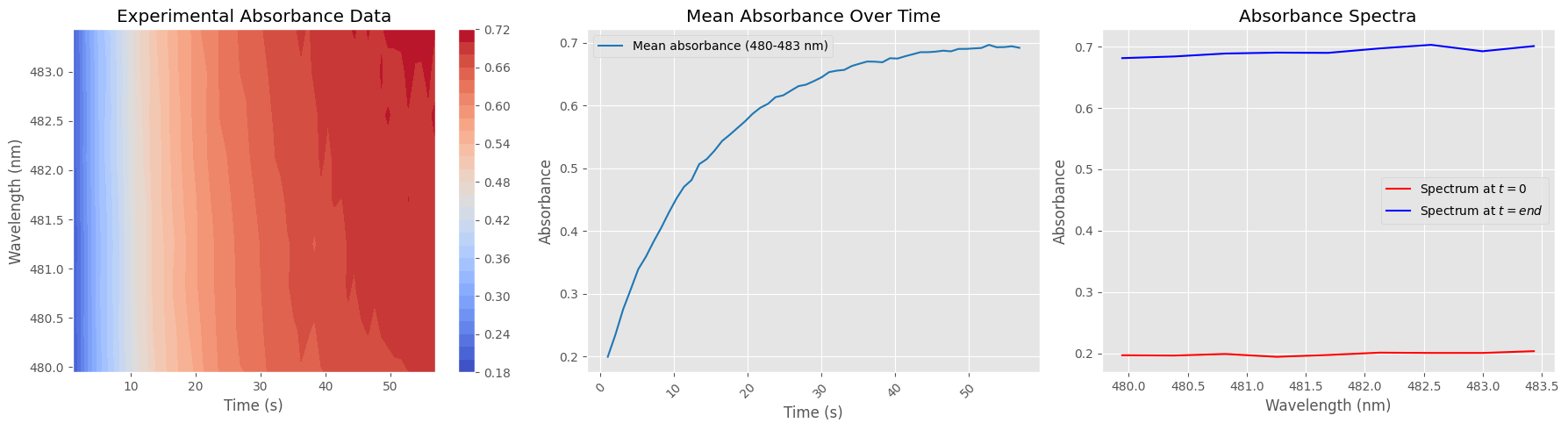
Data Cleaning and Absorbance Subset Preparation

This cell prepares the dataset for focused analysis by:

• Selecting a narrow wavelength range (e.g. 480–484 nm)

• Normalizing absorbance values

• Removing unwanted time points (first spectrum and last 300)

The resulting cleaned subset is suitable for targeted visualization or kinetic analysis.

# Define wavelength range of interest
wavelength_range = [480, 484]
idx_range = np.argmin(np.abs(wavelengths[:, None] - wavelength_range), axis=0)

# Extract and normalize absorbance data within the wavelength range
absorbance_subset = absorbance[:, idx_range[0]:idx_range[1]]
# absorbance_subset -= np.min(absorbance_subset)
wavelengths_subset = wavelengths[idx_range[0]:idx_range[1]]

# Filter out specific time points (e.g., first frame and last 300 entries)
# Adjust indices as needed
time_filter_indices = [0] + list(range(-300, 0))
absorbance_subset = np.delete(absorbance_subset, time_filter_indices, axis=0)
timestamps_filtered = np.delete(timestamps, time_filter_indices)

# Create subplots
fig, axs = plt.subplots(1, 3, figsize=(18, 5))

# --- 1. Absorbance Heatmap ---
X, Y = np.meshgrid(timestamps_filtered, wavelengths_subset)
contour = axs[0].contourf(X, Y, absorbance_subset.T, levels=30, cmap="coolwarm")
axs[0].set_title("Experimental Absorbance Data")
axs[0].set_xlabel("Time (s)")
axs[0].set_ylabel("Wavelength (nm)")
fig.colorbar(contour, ax=axs[0])

# --- 2. Absorbance Over Time (Averaged Across Wavelength Range) ---
mean_absorbance = np.mean(absorbance_subset, axis=1)
axs[1].plot(timestamps_filtered, mean_absorbance, label=f"Mean absorbance ({wavelengths_subset[0]:.0f}-{wavelengths_subset[-1]:.0f} nm)", color='tab:blue')
axs[1].set_title("Mean Absorbance Over Time")
axs[1].set_xlabel("Time (s)")
axs[1].set_ylabel("Absorbance")
axs[1].tick_params(axis="x", rotation=45)
axs[1].legend()
axs[1].grid(True)

# --- 3. Absorbance Spectrum at Start and End ---
axs[2].plot(wavelengths_subset, absorbance_subset[0, :], label="Spectrum at $t=0$", color='red')
axs[2].plot(wavelengths_subset, absorbance_subset[-1, :], label="Spectrum at $t=end$", color='blue')
axs[2].set_title("Absorbance Spectra")
axs[2].set_xlabel("Wavelength (nm)")
axs[2].set_ylabel("Absorbance")
axs[2].legend()
axs[2].grid(True)

plt.tight_layout()
plt.show()

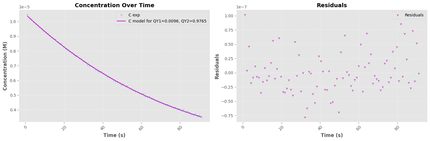
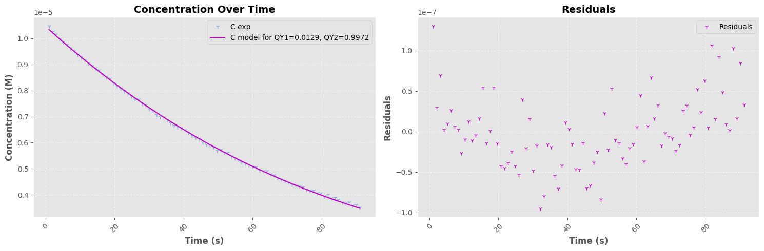
QY ON->OFF Regression

from scipy.integrate import solve_ivp
from scipy.optimize import curve_fit
import numpy as np
import matplotlib.pyplot as plt

# === Physics constants ===
h = 6.62607004 * 10 ** (-34)  # Planck's constant (J·s)
NA = 6.02214086 * 10 ** (23)  # Avogadro's number (mol^-1)
c_vaccum = 299792458  # Speed of light in vacuum (m/s)
wl = 505  # Wavelength (nm)
v = c_vaccum / (wl * 1e-9)  # Frequency (Hz)
volume = 23e-4  # Volume (L)
l = 1  # Path length (cm)
eps_on_482 = 65474  # Molar absorptivity (L·mol^-1·cm^-1)
eps_off_482 = 65  # Molar absorptivity (L·mol^-1·cm^-1)
eps_on_505 = 0.4166666667 * eps_on_482  # Adjusted molar absorptivity at 505
eps_off_505 = 0.4166666667 * eps_off_482  # Adjusted molar absorptivity at 505
I_w_list = [14.27e-3, 10.4e-3]  # Irradiance values (W/m^2)

# === Experimental data ===
# Assuming 'timestamps_filtered' and 'C_exp' are already defined

# === Initialize parameters ===
lpopt = []
for I_w in I_w_list:
    # Compute initial concentration based on experimental data
    C_exp = mean_absorbance / (eps_on_482 * l)
    C0 = C_exp[0]
    I_0 = I_w / (h * v * NA) / volume  # Photon irradiance (mol·L^-1·s^-1)

    # === ODE definition ===
    def dC_dt(t, C_ON, QY_ON2OFF, QY_OFF2ON):
        C_OFF = C0 - C_ON
        Iabs_ON = I_0 * (1 - np.exp(-eps_on_505 * C_ON * l * np.log(10)))
        Iabs_OFF = I_0 * (1 - np.exp(-eps_off_505 * C_OFF * l * np.log(10)))
        dCCF_deri = -QY_ON2OFF * Iabs_ON + QY_OFF2ON * Iabs_OFF
        return dCCF_deri

    # === Fitting function wrapper ===
    def model(t, QY_ON2OFF, QY_OFF2ON, offset):
        sol = solve_ivp(dC_dt, [t[0], t[-1]], [C0], args=(QY_ON2OFF, QY_OFF2ON), t_eval=t)
        if not sol.success:
            print("⚠️ ODE solver failed:", sol.message)
            return np.full_like(t, np.nan)
        return sol.y[0]+ offset

    # === Fit the model to the experimental data ===
    initial_guess = (0.001, 0.01, 0) # QY_ON2OFF, QY_OFF2ON, offset
    bounds = ([1e-4, 1e-4,-1], [0.2, 1,1]) # ([min1, min2, ...], [max1, max2, ...])
    popt, pcov = curve_fit(model, timestamps_filtered, C_exp, p0=initial_guess, bounds=bounds)

    # Extract fitted parameters and compute uncertainties
    uncertainties = np.sqrt(np.diag(pcov))
    lpopt.append(popt)
    print(f"=== Fit Results I={I_w:0.3e} W ===")
    for i, (coef, incert) in enumerate(zip(popt, uncertainties), start=1):
        print(f"Parameter {i}: {coef:.4f} ± {incert:.4f}")

    # Compute fitted values
    fitted_values = model(timestamps_filtered, *popt)

    # === Plotting ===
    fig, a = plt.subplots(1, 2, figsize=(15, 5))
    pastel_colors = ["m", "#f9955e", "#5080e0"]  # Mauve, orange, sky blue

    # First Plot - Concentration Over Time
    a[0].plot(timestamps_filtered, C_exp, "1", color=pastel_colors[2], label="C exp", alpha=0.6)
    a[0].plot(timestamps_filtered, fitted_values, "-", color=pastel_colors[0], label=f"C model for QY1={popt[0]:0.4f}, QY2={popt[1]:0.4f}")
    a[0].set_xlabel("Time (s)", fontsize=12, fontweight="bold")
    a[0].set_ylabel("Concentration (M)", fontsize=12, fontweight="bold")
    a[0].set_title("Concentration Over Time", fontsize=14, fontweight="bold")
    a[0].tick_params(axis="x", rotation=45)
    a[0].grid(linestyle="--", alpha=0.5)
    a[0].legend()

    # Second Plot - Residuals Over Time
    residuals = C_exp - fitted_values
    a[1].plot(timestamps_filtered, residuals, "1", color=pastel_colors[0], label="Residuals", alpha=0.9)
    a[1].set_xlabel("Time (s)", fontsize=12, fontweight="bold")
    a[1].set_ylabel("Residuals", fontsize=12, fontweight="bold")
    a[1].set_title("Residuals", fontsize=14, fontweight="bold")
    a[1].tick_params(axis="x", rotation=45)
    a[1].grid(linestyle="--", alpha=0.5)
    a[1].legend()

    plt.tight_layout()
    plt.show()

=== Fit Results I=1.427e-02 W ===
Parameter 1: 0.0096 ± 0.0001
Parameter 2: 0.9765 ± 0.0604
Parameter 3: -0.0000 ± 0.0000

=== Fit Results I=1.040e-02 W ===
Parameter 1: 0.0129 ± 0.0001
Parameter 2: 0.9972 ± 0.1030
Parameter 3: -0.0000 ± 0.0000

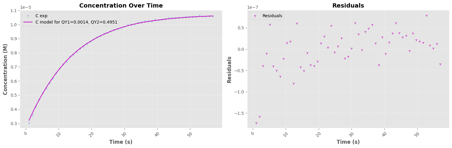
OFF -> ON

Load Experimental Switching Data

We begin by importing the required library and loading the actinometry measurement data from a CSV file. The dataset is stored in exp_data for further analysis

import pandas as pd

exp_data = pd.read_csv("DATA/prot1 OFF2ON.csv")

exp_data

	timestamp	cycle	type	186.85486	187.31995223015844	187.78500323297956	188.250012996982	188.71498151068454	189.17990876260572	189.64479474126426	...	1032.9632529736894	1033.3204920667242	1033.6776665334785	1034.034776362471	1034.3918215422202	1034.7488020612445	1035.1057179080635	1035.4625690711953	1035.8193555391586	1036.176077300472
0	2025-04-04 13:18:08.282867	1	zero	16.990556	24978.543889	33.859750	28.155778	33.738389	40.898694	38.956917	...	449.157472	435.807750	441.026278	435.443667	437.021361	448.672028	442.968056	451.463333	451.463333	451.463333
1	2025-04-04 13:18:36.280977	1	off	16.990556	24978.543889	45.038457	22.114691	31.823580	32.093272	49.623210	...	441.215062	443.642284	457.935926	446.339198	431.506173	445.530123	440.405988	450.384568	450.384568	450.384568
2	2025-04-04 13:18:37.311192	1	off	16.990556	24978.543889	31.823580	22.114691	42.341543	53.938272	58.792716	...	450.114877	450.384568	433.933395	450.923951	459.823765	444.721049	440.136296	459.823765	459.823765	459.823765
3	2025-04-04 13:18:38.352852	1	off	16.990556	24978.543889	54.477654	32.093272	37.487099	50.162593	59.332099	...	440.675679	443.372593	440.405988	445.530123	430.966790	437.439383	452.272407	429.078951	429.078951	429.078951
4	2025-04-04 13:18:39.383552	1	off	16.990556	24978.543889	39.644630	36.947716	37.756790	31.284198	61.219938	...	425.033580	463.599444	445.530123	451.193642	443.642284	453.620864	435.012160	434.203086	434.203086	434.203086
5	2025-04-04 13:18:40.416396	1	off	16.990556	24978.543889	19.687469	33.172037	42.341543	18.608704	38.296173	...	453.620864	446.878580	429.888025	438.518148	424.494198	439.327222	434.203086	451.193642	451.193642	451.193642
6	2025-04-04 13:18:41.449506	1	off	16.990556	24978.543889	28.317593	28.317593	30.205432	32.093272	42.611235	...	461.172222	433.933395	444.181667	432.315247	436.900000	419.909444	459.014691	448.766420	448.766420	448.766420
7	2025-04-04 13:18:42.486227	1	off	16.990556	24978.543889	40.453704	46.656605	20.766235	49.623210	65.265309	...	446.878580	450.114877	426.382037	429.348642	425.842654	437.169691	444.990741	449.036111	449.036111	449.036111
8	2025-04-04 13:18:43.531508	1	off	16.990556	24978.543889	32.093272	29.126667	25.890370	38.835556	52.859506	...	447.687654	445.260432	448.766420	435.281852	428.539568	415.594383	435.012160	425.303272	425.303272	425.303272
9	2025-04-04 13:18:44.565058	1	off	16.990556	24978.543889	31.014506	39.105247	51.780741	29.396358	63.107778	...	433.124321	458.205617	449.845185	447.687654	442.833210	439.057531	423.145741	439.866605	439.866605	439.866605
10	2025-04-04 13:18:45.595041	1	off	16.990556	24978.543889	22.923765	31.553889	55.017037	56.904877	46.926296	...	417.212531	438.787840	431.506173	446.069506	422.066975	419.370062	452.272407	428.539568	428.539568	428.539568
11	2025-04-04 13:18:46.624883	1	off	16.990556	24978.543889	32.093272	27.238827	28.047901	29.126667	47.735370	...	431.506173	435.821235	436.630309	460.363148	428.809259	440.405988	453.890556	438.787840	438.787840	438.787840
12	2025-04-04 13:18:47.658044	1	off	16.990556	24978.543889	26.699444	39.105247	36.678025	15.642099	52.050432	...	454.429938	436.360617	442.024136	430.157716	414.245926	442.293827	455.239012	451.463333	451.463333	451.463333
13	2025-04-04 13:18:48.687960	1	off	16.990556	24978.543889	28.856975	48.005062	20.226852	31.553889	71.198519	...	450.384568	430.697099	435.281852	444.451358	427.730494	423.685123	427.191111	448.766420	448.766420	448.766420
14	2025-04-04 13:18:49.728411	1	off	16.990556	24978.543889	46.386914	16.720864	24.811605	49.353519	66.074383	...	445.530123	414.515617	448.227037	417.482222	448.496728	453.351173	438.248457	452.002716	452.002716	452.002716
15	2025-04-04 13:18:50.761486	1	off	16.990556	24978.543889	43.420309	33.711420	38.835556	42.071852	33.441728	...	426.112346	430.697099	435.551543	419.639753	442.293827	444.721049	445.799815	443.372593	443.372593	443.372593
16	2025-04-04 13:18:51.804446	1	off	16.990556	24978.543889	49.029889	31.553889	54.612500	54.855222	56.797000	...	444.424389	446.366167	434.472778	437.870889	425.249333	440.055389	437.142722	441.754444	441.754444	441.754444
17	2025-04-04 13:18:52.839511	1	off	16.990556	24978.543889	48.274753	22.923765	25.890370	37.756790	51.241358	...	440.405988	435.281852	447.417963	419.370062	424.224506	453.351173	436.900000	436.360617	436.360617	436.360617
18	2025-04-04 13:18:53.878424	1	off	16.990556	24978.543889	42.476389	30.097556	45.146333	61.894167	50.971667	...	430.346500	416.754056	439.569944	423.793000	442.968056	466.269389	450.735167	458.259556	458.259556	458.259556
19	2025-04-04 13:18:54.916155	1	off	16.990556	24978.543889	25.890370	25.890370	51.780741	30.475123	61.489630	...	437.978765	442.024136	432.584938	438.518148	450.654259	449.575494	460.632840	452.272407	452.272407	452.272407
20	2025-04-04 13:18:55.948033	1	off	16.990556	24978.543889	59.601790	38.296173	29.666049	50.162593	24.541914	...	444.181667	463.599444	450.114877	422.606358	468.184198	443.102901	443.642284	439.596914	439.596914	439.596914
21	2025-04-04 13:18:56.982133	1	off	16.990556	24978.543889	30.744815	42.611235	33.441728	31.823580	69.040988	...	418.021605	428.000185	425.572963	442.833210	442.024136	445.260432	419.639753	460.363148	460.363148	460.363148
22	2025-04-04 13:18:58.028200	1	off	16.990556	24978.543889	27.427611	38.835556	20.145944	31.553889	34.466556	...	440.298111	455.589611	441.269000	441.026278	425.006611	456.803222	439.569944	443.938944	443.938944	443.938944
23	2025-04-04 13:18:59.065314	1	off	16.990556	24978.543889	46.117222	22.654074	29.666049	25.890370	47.195988	...	450.923951	437.169691	430.966790	448.496728	440.405988	447.417963	440.945370	438.248457	438.248457	438.248457
24	2025-04-04 13:19:00.095774	1	off	16.990556	24978.543889	27.427611	19.175056	21.845000	35.437444	56.311556	...	459.230444	430.346500	448.550667	450.007000	441.511722	440.055389	448.065222	437.628167	437.628167	437.628167
25	2025-04-04 13:19:01.128261	1	off	16.990556	24978.543889	37.217407	14.293642	28.317593	41.532469	47.735370	...	436.090926	438.518148	440.405988	449.575494	436.630309	434.472778	456.857160	436.900000	436.900000	436.900000
26	2025-04-04 13:19:02.160391	1	off	16.990556	24978.543889	38.350111	26.942167	51.699833	39.321000	55.097944	...	447.579778	415.055000	426.220222	448.065222	453.890556	439.084500	436.171833	442.968056	442.968056	442.968056
27	2025-04-04 13:19:03.202006	1	off	16.990556	24978.543889	17.529938	40.993086	41.532469	46.926296	44.499074	...	450.114877	456.048086	430.427407	442.563519	452.002716	427.460802	436.090926	438.248457	438.248457	438.248457
28	2025-04-04 13:19:04.242210	1	off	16.990556	24978.543889	40.777333	30.583000	21.845000	37.864667	57.767889	...	445.395278	432.045556	443.210778	457.531389	459.230444	443.453500	444.181667	436.414556	436.414556	436.414556
29	2025-04-04 13:19:05.280109	1	off	16.990556	24978.543889	39.914321	42.341543	25.890370	47.735370	55.286728	...	420.988210	461.981296	433.933395	445.530123	432.315247	430.966790	468.184198	435.551543	435.551543	435.551543
30	2025-04-04 13:19:06.334964	1	off	16.990556	24978.543889	47.330833	22.815889	44.418167	56.797000	54.127056	...	436.171833	445.395278	470.152944	423.550278	433.744611	440.055389	435.686389	432.288278	432.288278	432.288278
31	2025-04-04 13:19:07.367506	1	off	16.990556	24978.543889	37.217407	27.778210	31.553889	29.935741	46.117222	...	450.654259	430.427407	424.763889	450.654259	428.539568	447.957346	458.205617	414.515617	414.515617	414.515617
32	2025-04-04 13:19:08.397854	1	off	16.990556	24978.543889	19.417778	21.602278	53.156167	47.816278	58.738778	...	425.734778	431.074667	465.055778	443.453500	457.774111	450.007000	429.375611	440.055389	440.055389	440.055389
33	2025-04-04 13:19:09.427097	1	off	16.990556	24978.543889	31.014506	16.990556	30.475123	34.250802	61.759321	...	450.923951	466.835741	455.778395	454.969321	448.496728	444.181667	456.048086	430.697099	430.697099	430.697099
34	2025-04-04 13:19:10.459716	1	off	16.990556	24978.543889	42.880926	25.350988	49.353519	52.859506	56.904877	...	453.620864	463.329753	446.608889	450.384568	426.382037	446.878580	425.033580	424.763889	424.763889	424.763889
35	2025-04-04 13:19:11.491974	1	off	16.990556	24978.543889	48.274753	23.732840	23.193457	43.420309	68.231914	...	464.138827	446.878580	434.472778	427.191111	429.348642	449.575494	443.911975	432.045556	432.045556	432.045556
36	2025-04-04 13:19:12.537711	1	off	16.990556	24978.543889	26.429753	11.866420	58.253333	47.195988	54.477654	...	428.539568	410.200556	443.911975	435.281852	435.281852	451.193642	427.460802	444.990741	444.990741	444.990741
37	2025-04-04 13:19:13.572105	1	off	16.990556	24978.543889	39.105247	12.405802	27.508519	33.711420	52.050432	...	438.787840	444.721049	435.551543	450.384568	452.811790	440.405988	443.911975	448.496728	448.496728	448.496728
38	2025-04-04 13:19:14.604002	1	off	16.990556	24978.543889	28.047901	20.766235	52.589815	32.902346	50.971667	...	430.157716	430.966790	440.675679	451.463333	422.336667	423.145741	442.293827	432.045556	432.045556	432.045556
39	2025-04-04 13:19:15.637091	1	off	16.990556	24978.543889	24.272222	48.544444	36.947716	49.623210	57.174568	...	441.754444	445.260432	443.372593	440.136296	447.417963	464.408519	452.002716	450.654259	450.654259	450.654259
40	2025-04-04 13:19:16.672483	1	off	16.990556	24978.543889	30.744815	46.656605	33.172037	44.229383	35.059877	...	442.024136	443.911975	449.305802	473.578025	440.945370	427.730494	444.990741	448.496728	448.496728	448.496728
41	2025-04-04 13:19:17.706073	1	off	16.990556	24978.543889	26.699444	25.485833	38.835556	39.563722	34.223833	...	427.919278	464.570333	442.968056	430.589222	443.210778	447.822500	436.414556	434.230056	434.230056	434.230056
42	2025-04-04 13:19:18.742677	1	off	16.990556	24978.543889	42.341543	25.350988	37.217407	48.814136	53.398889	...	433.663704	434.742469	429.618333	416.673148	452.002716	450.384568	427.191111	437.709074	437.709074	437.709074
43	2025-04-04 13:19:19.775702	1	off	16.990556	24978.543889	19.957160	19.148086	30.205432	35.059877	60.950247	...	436.630309	451.733025	443.372593	444.721049	439.057531	449.575494	452.542099	426.382037	426.382037	426.382037
44	2025-04-04 13:19:20.805906	1	off	16.990556	24978.543889	28.856975	18.608704	24.811605	34.250802	48.274753	...	453.890556	457.126852	443.102901	454.429938	430.427407	456.587469	459.014691	438.248457	438.248457	438.248457
45	2025-04-04 13:19:21.836857	1	off	16.990556	24978.543889	39.374938	45.308148	22.923765	46.926296	51.780741	...	432.854630	438.248457	461.981296	421.257901	444.990741	424.763889	445.260432	432.854630	432.854630	432.854630
46	2025-04-04 13:19:22.871144	1	off	16.990556	24978.543889	46.117222	30.825722	21.359556	50.971667	54.612500	...	439.812667	450.007000	443.210778	427.919278	446.123444	436.657278	435.686389	438.113611	438.113611	438.113611
47	2025-04-04 13:19:23.908302	1	off	16.990556	24978.543889	36.678025	40.184012	36.678025	38.026481	49.623210	...	456.857160	446.339198	452.002716	449.036111	438.248457	430.966790	444.990741	429.078951	429.078951	429.078951
48	2025-04-04 13:19:24.941178	1	off	16.990556	24978.543889	42.476389	23.058611	19.417778	60.437833	46.359944	...	444.181667	419.666722	431.074667	431.802833	450.977889	439.327222	444.667111	449.764278	449.764278	449.764278
49	2025-04-04 13:19:25.976058	1	off	16.990556	24978.543889	51.511049	24.272222	33.711420	52.320123	46.656605	...	439.327222	427.191111	442.293827	436.090926	438.787840	457.396543	440.945370	476.005247	476.005247	476.005247
50	2025-04-04 13:19:27.008444	1	off	16.990556	24978.543889	39.105247	31.823580	39.374938	48.544444	43.959691	...	465.756975	429.888025	436.090926	446.069506	452.811790	452.272407	422.606358	450.923951	450.923951	450.923951
51	2025-04-04 13:19:28.045717	1	off	16.990556	24978.543889	49.892901	51.511049	49.083827	28.856975	68.501605	...	464.678210	440.136296	429.618333	453.081481	443.372593	436.900000	429.078951	444.451358	444.451358	444.451358
52	2025-04-04 13:19:29.076808	1	off	16.990556	24978.543889	31.553889	12.405802	43.690000	38.565864	67.153148	...	446.069506	463.869136	433.933395	441.754444	440.136296	431.775864	449.575494	435.012160	435.012160	435.012160
53	2025-04-04 13:19:30.113538	1	off	16.990556	24978.543889	45.308148	30.475123	34.520494	14.023951	46.117222	...	460.632840	444.181667	438.248457	440.405988	437.978765	444.451358	427.191111	440.405988	440.405988	440.405988
54	2025-04-04 13:19:31.146010	1	off	16.990556	24978.543889	54.207963	27.508519	37.217407	35.599259	51.780741	...	447.687654	442.024136	470.341728	459.554074	424.494198	434.742469	444.181667	436.360617	436.360617	436.360617
55	2025-04-04 13:19:32.180604	1	off	16.990556	24978.543889	30.475123	33.981111	43.690000	40.993086	52.050432	...	429.348642	444.990741	419.909444	431.506173	430.427407	437.709074	461.981296	444.181667	444.181667	444.181667
56	2025-04-04 13:19:33.213159	1	off	16.990556	24978.543889	35.329568	29.666049	16.990556	37.217407	57.983642	...	433.124321	441.484753	441.484753	455.778395	451.463333	437.439383	442.563519	438.787840	438.787840	438.787840
57	2025-04-04 13:19:46.247957	1	static	16.990556	24978.543889	42.840472	38.350111	28.277139	32.767500	58.010611	...	426.220222	443.817583	446.123444	449.036111	430.467861	437.264083	419.545361	451.220611	451.220611	451.220611

58 rows × 2051 columns

import numpy as np

intensities=np.array(exp_data[(exp_data["type"] != "zero") & (exp_data["type"] != "static")].iloc[:, 3:], dtype=np.float64)
static=np.array(exp_data[(exp_data["type"]== "static")].iloc[:, 3:], dtype=np.float64)[0]
zero=np.array(exp_data[(exp_data["type"]== "zero")].iloc[:, 3:], dtype=np.float64)[0]
wavelengths = np.array(exp_data.columns[3:], dtype=np.float64)
timestamps = pd.to_datetime(exp_data["timestamp"][(exp_data["type"] != "zero") & (exp_data["type"] != "static")]) # Convert timestamp strings to datetime objects
timestamps = np.array((timestamps - timestamps.iloc[0]).dt.total_seconds()) # Convert to seconds since the first timestamp

def compute_absorbance(intensities: np.ndarray, static: np.ndarray, zero: np.ndarray) -> np.ndarray:
    EPS = 1e-12
    num = intensities - static
    den = np.maximum(zero - static, EPS)  # Éviter division par zéro
    absorbance = -np.log10(np.maximum(num / den, EPS))  # Éviter log(0) ou log(négatif)
    return absorbance

absorbance = compute_absorbance(intensities, static, zero)

Show code cell source Hide code cell source

import matplotlib.pyplot as plt
import matplotlib.cm as cm
# Set global style
plt.style.use("ggplot")  # Clean style

fig, axs = plt.subplots(1, 3, figsize=(18, 5))
fig.suptitle("Spectral Analysis", fontsize=16)

# --- Intensity Plot ---
axs[0].plot(wavelengths, intensities[0, :], label=f"I at t = {timestamps[0]:.0f} s", linewidth=2)
axs[0].plot(wavelengths, intensities[len(intensities)//2, :], label=f"I at t = {timestamps[len(intensities)//2]:.0f} s", linewidth=2)
axs[0].plot(wavelengths, intensities[-1, :], label=f"I at t = {timestamps[-1]:.0f} s", linewidth=2)
axs[0].plot(wavelengths, static, '--', label="Static", linewidth=2)
axs[0].plot(wavelengths, zero, '--', label="Zero", linewidth=2)
axs[0].set_title("Intensity over Wavelength")
axs[0].set_xlabel("Wavelength (nm)")
axs[0].set_ylabel("Intensity")
axs[0].legend()
axs[0].grid(True, which='major', linestyle='--', linewidth=0.6, color='gray', alpha=0.5, zorder=0)
axs[0].minorticks_on()
axs[0].grid(True, which='minor', linestyle=':', linewidth=0.3, color='lightgray', alpha=0.4, zorder=0)
# --- Absorbance Plot ---
axs[1].plot(wavelengths, absorbance[0, :], label=f"t = {timestamps[0]:.0f} s", linewidth=2)
axs[1].plot(wavelengths, absorbance[len(absorbance)//2, :], label=f"t = {timestamps[len(absorbance)//2]:.0f} s", linewidth=2)
axs[1].plot(wavelengths, absorbance[-1, :], label=f"t = {timestamps[-1]:.0f} s", linewidth=2)
axs[1].set_title("Absorbance over Wavelength")
axs[1].set_xlabel("Wavelength (nm)")
axs[1].set_ylabel("Absorbance")
axs[1].set_ylim(-0.4, 2)
axs[1].legend()
axs[1].grid(True, which='major', linestyle='--', linewidth=0.6, color='gray', alpha=0.5, zorder=0)
axs[1].minorticks_on()
axs[1].grid(True, which='minor', linestyle=':', linewidth=0.3, color='lightgray', alpha=0.4, zorder=0)
# --- Absorbance vs Time Plot ---
WL = [482, 408]
idxs = [np.argmin(np.abs(wavelengths - wl)) for wl in WL]

for i, idx in enumerate(idxs):
    axs[2].plot(timestamps, absorbance[:, idx], label=f"{wavelengths[idx]:.0f} nm", linewidth=2)

axs[2].set_title("Absorbance over Time")
axs[2].set_xlabel("Time (s)")
axs[2].set_ylabel("Absorbance")
axs[2].legend()
axs[2].grid(True, which='major', linestyle='--', linewidth=0.6, color='gray', alpha=0.5, zorder=0)
axs[2].minorticks_on()
axs[2].grid(True, which='minor', linestyle=':', linewidth=0.3, color='lightgray', alpha=0.4, zorder=0)
plt.tight_layout(rect=[0, 0, 1, 0.95])
plt.show()

# la premiere mesure doit etre viré

# Define wavelength range of interest
wavelength_range = [480, 484]
idx_range = np.argmin(np.abs(wavelengths[:, None] - wavelength_range), axis=0)

# Extract and normalize absorbance data within the wavelength range
absorbance_subset = absorbance[:, idx_range[0]:idx_range[1]]
# absorbance_subset -= np.min(absorbance_subset)
wavelengths_subset = wavelengths[idx_range[0]:idx_range[1]]

# Filter out specific time points (e.g., first frame and last 300 entries)
# Adjust indices as needed
time_filter_indices = [0] #+ list(range(-45, 0))
absorbance_subset = np.delete(absorbance_subset, time_filter_indices, axis=0)
timestamps_filtered = np.delete(timestamps, time_filter_indices)

# Create subplots
fig, axs = plt.subplots(1, 3, figsize=(18, 5))

# --- 1. Absorbance Heatmap ---
X, Y = np.meshgrid(timestamps_filtered, wavelengths_subset)
contour = axs[0].contourf(X, Y, absorbance_subset.T, levels=30, cmap="coolwarm")
axs[0].set_title("Experimental Absorbance Data")
axs[0].set_xlabel("Time (s)")
axs[0].set_ylabel("Wavelength (nm)")
fig.colorbar(contour, ax=axs[0])

# --- 2. Absorbance Over Time (Averaged Across Wavelength Range) ---
mean_absorbance = np.mean(absorbance_subset, axis=1)
axs[1].plot(timestamps_filtered, mean_absorbance, label=f"Mean absorbance ({wavelengths_subset[0]:.0f}-{wavelengths_subset[-1]:.0f} nm)", color='tab:blue')
axs[1].set_title("Mean Absorbance Over Time")
axs[1].set_xlabel("Time (s)")
axs[1].set_ylabel("Absorbance")
axs[1].tick_params(axis="x", rotation=45)
axs[1].legend()
axs[1].grid(True)

# --- 3. Absorbance Spectrum at Start and End ---
axs[2].plot(wavelengths_subset, absorbance_subset[0, :], label="Spectrum at $t=0$", color='red')
axs[2].plot(wavelengths_subset, absorbance_subset[-1, :], label="Spectrum at $t=end$", color='blue')
axs[2].set_title("Absorbance Spectra")
axs[2].set_xlabel("Wavelength (nm)")
axs[2].set_ylabel("Absorbance")
axs[2].legend()
axs[2].grid(True)

plt.tight_layout()
plt.show()

from scipy.integrate import solve_ivp
from scipy.optimize import curve_fit
import numpy as np
import matplotlib.pyplot as plt

# === Physics constants ===
h = 6.62607004 * 10 ** (-34)  # Planck's constant (J·s)
NA = 6.02214086 * 10 ** (23)  # Avogadro's number (mol^-1)
c_vaccum = 299792458  # Speed of light in vacuum (m/s)
wl = 405  # Wavelength (nm)
v = c_vaccum / (wl * 1e-9)  # Frequency (Hz)
volume = 23e-4  # Volume (L)
l = 1  # Path length (cm)

eps_on_482 = 65474
eps_off_482 = 65
eps_on_405 = 0.1847826087*eps_on_482
eps_off_405 = 25343

I_w_list = [ 3.8e-3 ] # No actinometry for 405nm LED

# === Experimental data ===
# Assuming 'timestamps_filtered' and 'C_exp' are already defined

# === Initialize parameters ===
lpopt = []
for I_w in I_w_list:
    # Compute initial concentration based on experimental data
    C_exp = mean_absorbance / (eps_on_482 * l)
    C0 = C_exp[-1]
    I_0 = I_w / (h * v * NA) / volume  # Photon irradiance (mol·L^-1·s^-1)

    # === ODE definition ===
    def dC_dt(t, C_ON, QY_ON2OFF, QY_OFF2ON):
        C_OFF = C0 - C_ON
        Iabs_ON = I_0 * (1 - np.exp(-eps_on_405 * C_ON * l * np.log(10)))
        Iabs_OFF = I_0 * (1 - np.exp(-eps_on_405 * C_OFF * l * np.log(10)))
        dCCF_deri = -QY_ON2OFF * Iabs_ON + QY_OFF2ON * Iabs_OFF
        return dCCF_deri

    # === Fitting function wrapper ===
    def model(t, QY_ON2OFF, QY_OFF2ON, offset):
        sol = solve_ivp(dC_dt, [t[0], t[-1]], [C_exp[0]], args=(QY_ON2OFF, QY_OFF2ON), t_eval=t)
        if not sol.success:
            print("⚠️ ODE solver failed:", sol.message)
            return np.full_like(t, np.nan)
        return sol.y[0]+ offset

    # === Fit the model to the experimental data ===
    initial_guess = (0.001, 0.2, 0) # QY_ON2OFF, QY_OFF2ON, offset
    bounds = ([1e-4, 1e-4,-1], [0.1, 1,1]) # ([min1, min2, ...], [max1, max2, ...])
    popt, pcov = curve_fit(model, timestamps_filtered, C_exp, p0=initial_guess, bounds=bounds)

    # Extract fitted parameters and compute uncertainties
    uncertainties = np.sqrt(np.diag(pcov))
    lpopt.append(popt)
    print(f"=== Fit Results I={I_w:0.3e} W ===")
    for i, (coef, incert) in enumerate(zip(popt, uncertainties), start=1):
        print(f"Parameter {i}: {coef:.4f} ± {incert:.4f}")

    # Compute fitted values
    fitted_values = model(timestamps_filtered, *popt)

    # === Plotting ===
    fig, a = plt.subplots(1, 2, figsize=(15, 5))
    pastel_colors = ["m", "#f9955e", "#5080e0"]  # Mauve, orange, sky blue

    # First Plot - Concentration Over Time
    a[0].plot(timestamps_filtered, C_exp, "1", color=pastel_colors[2], label="C exp", alpha=0.6)
    a[0].plot(timestamps_filtered, fitted_values, "-", color=pastel_colors[0], label=f"C model for QY1={popt[0]:0.4f}, QY2={popt[1]:0.4f}")
    a[0].set_xlabel("Time (s)", fontsize=12, fontweight="bold")
    a[0].set_ylabel("Concentration (M)", fontsize=12, fontweight="bold")
    a[0].set_title("Concentration Over Time", fontsize=14, fontweight="bold")
    a[0].tick_params(axis="x", rotation=45)
    a[0].grid(linestyle="--", alpha=0.5)
    a[0].legend()

    # Second Plot - Residuals Over Time
    residuals = C_exp - fitted_values
    a[1].plot(timestamps_filtered, residuals, "1", color=pastel_colors[0], label="Residuals", alpha=0.9)
    a[1].set_xlabel("Time (s)", fontsize=12, fontweight="bold")
    a[1].set_ylabel("Residuals", fontsize=12, fontweight="bold")
    a[1].set_title("Residuals", fontsize=14, fontweight="bold")
    a[1].tick_params(axis="x", rotation=45)
    a[1].grid(linestyle="--", alpha=0.5)
    a[1].legend()

    plt.tight_layout()
    plt.show()

=== Fit Results I=3.800e-03 W ===
Parameter 1: 0.0014 ± 0.0013
Parameter 2: 0.4951 ± 0.0044
Parameter 3: 0.0000 ± 0.0000