Photofatigue Measurements

1. Import Data and Preprocess for Photofatigue Measurements

In this first step, we import the necessary experimental data from a CSV file.

• Timestamp filtering: Only data after 2025-04-08 is used for analysis.

import pandas as pd

# Load experimental data
exp_data = pd.read_csv("DATA/Spectrumsfatigue.csv")

# Filter data to include only entries after a specific timestamp
exp_data = exp_data[exp_data["timestamp"] > "2025-04-08"]

# Display the filtered dataset
exp_data

	timestamp	cycle	type	186.85486	187.31995223015844	187.78500323297956	188.250012996982	188.71498151068454	189.17990876260572	189.64479474126426	...	1032.9632529736894	1033.3204920667242	1033.6776665334785	1034.034776362471	1034.3918215422202	1034.7488020612445	1035.1057179080635	1035.4625690711953	1035.8193555391586	1036.176077300472
863	2025-04-08 09:38:38.241780	0	zero	16.990556	24978.543889	347.456861	334.956667	350.490889	359.228889	371.365000	...	759.235111	750.739833	755.958361	750.497111	755.715639	744.793139	754.866111	767.123583	767.123583	767.123583
864	2025-04-08 09:39:44.486116	1	on	16.990556	24978.543889	352.796750	356.680306	352.796750	362.262917	357.772556	...	746.977639	739.453250	747.220361	749.162139	757.050611	759.720556	766.516778	749.768944	749.768944	749.768944
865	2025-04-08 09:40:19.529467	1	off	16.990556	24978.543889	358.986167	352.554028	341.631528	371.365000	379.010750	...	750.133028	751.468000	743.458167	763.968194	746.128111	754.866111	750.254389	757.414694	757.414694	757.414694
866	2025-04-08 09:40:25.564251	1	static	16.990556	24978.543889	357.408472	358.500722	346.850056	365.418306	381.802056	...	757.293333	741.273667	763.361389	770.643056	762.754583	767.244944	753.773861	760.327361	760.327361	760.327361
867	2025-04-08 09:40:40.608372	2	on	16.990556	24978.543889	365.054222	348.063667	360.199778	361.170667	372.093167	...	748.676694	744.914500	757.293333	764.089556	756.079722	753.167056	758.992389	746.249472	746.249472	746.249472
...	...	...	...	...	...	...	...	...	...	...	...	...	...	...	...	...	...	...	...	...	...
1546	2025-04-08 13:12:50.290246	228	off	16.990556	24978.543889	133.861306	130.705917	121.361111	138.230306	137.987583	...	527.192667	531.561667	525.979056	522.823667	544.425944	529.255806	546.489083	529.741250	529.741250	529.741250
1547	2025-04-08 13:12:56.349038	228	static	16.990556	24978.543889	114.928972	119.540694	125.001944	127.065083	139.686639	...	534.595694	513.721583	545.032750	522.459583	520.153722	537.629722	546.246361	533.867528	533.867528	533.867528
1548	2025-04-08 13:13:11.473565	229	on	16.990556	24978.543889	118.448444	124.880583	126.094194	121.482472	145.026528	...	532.047111	529.377167	523.915917	534.959778	522.338222	530.712139	535.930667	543.455056	543.455056	543.455056
1549	2025-04-08 13:13:46.542295	229	off	16.990556	24978.543889	122.332000	109.103639	114.564889	131.070000	147.332389	...	528.527639	536.658833	526.221778	529.983972	530.712139	527.678111	536.294750	537.022917	537.022917	537.022917
1550	2025-04-08 13:13:52.603917	229	static	16.990556	24978.543889	117.113472	109.710444	104.491917	120.754306	151.580028	...	547.824056	526.585861	545.275472	530.590778	553.285306	511.051639	528.891722	517.241056	517.241056	517.241056

688 rows × 2051 columns

2. Data Preparation: Intensity Arrays & Absorbance Calculation

Now, we prepare the intensity data based on the “on”, “off”, “static”, and “zero” conditions. These intensity values will be used to compute the absorbance values.

• Intensity arrays: Data for “on” and “off” states are extracted, along with the static and zero intensity references.

• Absorbance formula: Absorbance is calculated from the intensity data using the formula:

$$ A = -\log_{10}\left(\frac{I_{\text{on}} - I_{\text{static}}}{I_{\text{zero}} - I_{\text{static}}}\right) $$

where:

• $I_{\text{on}}$ is the intensity during the “on” state,

• $I_{\text{static}}$ is the static reference intensity,

• $I_{\text{zero}}$ is the zero intensity reference.

import numpy as np

# Extract relevant data for 'on', 'off', 'static', and 'zero' conditions
I_on = np.array(exp_data[exp_data["type"] == "on"].iloc[:, 3:], dtype=np.float64)
I_off = np.array(exp_data[exp_data["type"] == "off"].iloc[:, 3:], dtype=np.float64)
static = np.array(exp_data[(exp_data["type"] == "static")].iloc[:, 3:], dtype=np.float64)
zero = np.array(exp_data[(exp_data["type"] == "zero")].iloc[:, 3:], dtype=np.float64)

# Extract wavelengths (assumed to be in columns from 3 onward)
wavelengths = np.array(exp_data.columns[3:], dtype=np.float64)

# Convert timestamps to seconds since the first "on" timestamp
t_on = pd.to_datetime(exp_data["timestamp"][exp_data["type"] == "on"])
t_on = np.array((t_on - t_on.iloc[0]).dt.total_seconds())

t_off = pd.to_datetime(exp_data["timestamp"][exp_data["type"] == "off"])
t_off = np.array((t_off - t_off.iloc[0]).dt.total_seconds())

# Function to calculate absorbance
def compute_absorbance(intensities: np.ndarray, static: np.ndarray, zero: np.ndarray) -> np.ndarray:
    EPS = 1e-12  # Small epsilon to avoid division by zero
    num = intensities - static
    den = np.maximum(zero - static, EPS)  # Prevent division by zero
    absorbance = -np.log10(np.maximum(num / den, EPS))  # Avoid log(0) or negative
    return absorbance

# Calculate absorbance for "on" and "off" intensities
A_on = compute_absorbance(I_on, static, zero)
A_off = compute_absorbance(I_off, static, zero)

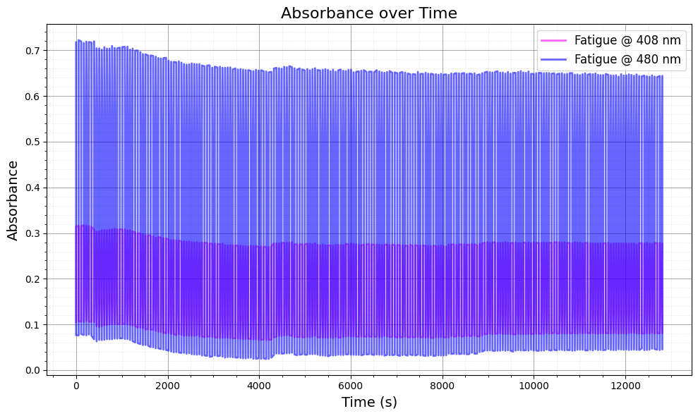
3. Plot Absorbance vs Time for Selected Wavelengths

In this section, we visualize the absorbance data over time for selected wavelengths (408 nm and 480 nm). This helps to assess the photofatigue effects at these specific wavelengths.

• Plotting: We plot the absorbance for both “on” and “off” conditions for each of the selected wavelengths.

The absorbance is shown as a function of time for the given wavelength range.

import matplotlib.pyplot as plt

# Define target wavelengths (in nm)
wavelength_target = [408, 480]
wavelength_idxs = np.argmin(np.abs(wavelengths[:, None] - np.array(wavelength_target)), axis=0)

# Create the figure and axis
fig, ax = plt.subplots(figsize=(10, 6))
colors = [["#FF00FF", "#412544"], ["blue", "red"]]  # Colors for different wavelengths

# Plot absorbance over time for selected wavelengths
for i, idx in enumerate(wavelength_idxs):
    t_combined = np.concatenate([t_on, t_off])  # Combine on and off times
    A_combined = np.concatenate([A_on[:, idx], A_off[:, idx]])  # Combine on and off absorbance

    # Sort by time
    sorted_indices = np.argsort(t_combined)
    t_sorted = t_combined[sorted_indices]
    A_sorted = A_combined[sorted_indices]

    # Plot combined data
    ax.plot(
        t_sorted, A_sorted,
        label=f"Fatigue @ {wavelengths[idx]:.0f} nm",
        color=colors[i][0],  # Color for each wavelength
        linewidth=2,
        alpha=0.6,
    )

# Set axis labels and title
ax.set_title("Absorbance over Time", fontsize=16)
ax.set_xlabel("Time (s)", fontsize=14)
ax.set_ylabel("Absorbance", fontsize=14)

# Add legend and grid
ax.legend(fontsize=12)
ax.minorticks_on()
ax.grid(which='major', linestyle='-', linewidth=0.6, color='black', alpha=0.4)
ax.grid(which='minor', linestyle=':', linewidth=0.4, color='black', alpha=0.2)

# Ensure layout is tidy
ax.set_axisbelow(True)
plt.tight_layout()
plt.show()

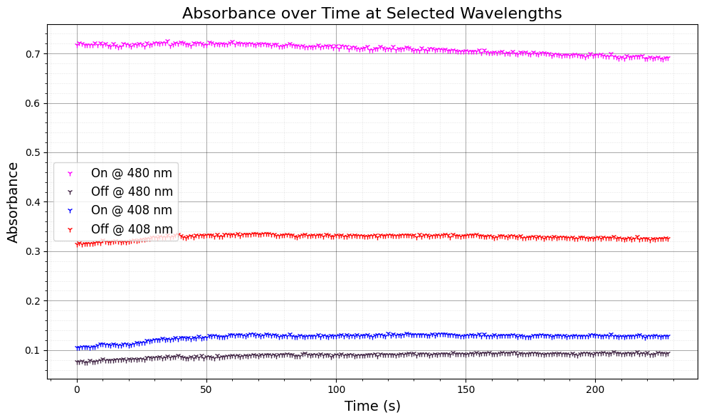
4. Adjust Absorbance for Offset and Plot

Here, we adjust the absorbance data for the “on” and “off” conditions by subtracting the absorbance at a reference wavelength (550 nm) to account for baseline shifts. This correction ensures a more accurate comparison between wavelengths.

# Define target wavelengths
wavelength_target = [480, 408]
wavelength_idxs = np.argmin(np.abs(wavelengths[:, None] - np.array(wavelength_target)), axis=0)

# Reference wavelength for adjustment (e.g., 550 nm)
wlt = 550
id2 = np.argmin(np.abs(wavelengths[:, None] - np.array(wlt)))

# Create the figure and axis
fig, ax = plt.subplots(figsize=(10, 6))
colors = [["#FF00FF", "#412544"], ["blue", "red"]]  # Colors for different wavelengths

# Plot absorbance over time with adjustments
for i, idx in enumerate(wavelength_idxs):
    # Adjust "on" absorbance data
    ax.plot(
        A_on[:, idx] - 1 * (A_on[:, id2] - np.min(A_on[0, id2])), "1",
        label=f"On @ {wavelengths[idx]:.0f} nm",
        color=colors[i][0],
        linewidth=2
    )

    # Adjust "off" absorbance data
    ax.plot(
        A_off[:, idx] - 1 * (A_off[:, id2] - np.min(A_off[0, id2])), "1",
        label=f"Off @ {wavelengths[idx]:.0f} nm",
        color=colors[i][1],
        linewidth=2
    )

# Set axis labels and title
ax.set_title("Absorbance over Time at Selected Wavelengths", fontsize=16)
ax.set_xlabel("Time (s)", fontsize=14)
ax.set_ylabel("Absorbance", fontsize=14)

# Add legend and grid
ax.legend(fontsize=12)
ax.minorticks_on()
ax.grid(which='major', linestyle='-', linewidth=0.6, color='black', alpha=0.4)
ax.grid(which='minor', linestyle=':', linewidth=0.4, color='black', alpha=0.2)

# Ensure layout is tidy
ax.set_axisbelow(True)
plt.tight_layout()
plt.show()

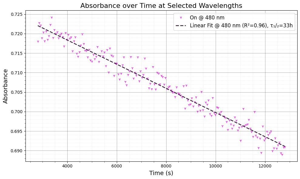
5. Linear Fit and Time Constant Estimation

We now perform a linear regression on the absorbance data to estimate the time constant (τ) for the photofatigue process. This is calculated by fitting the absorbance data to a linear model, where the slope gives us the decay rate.

• Linear regression: We fit the absorbance data after the initial part of the signal (after 50 seconds) to a linear model.

• Time constant: From the linear regression results, we calculate the time constant as $( \tau_{1/2} = \frac{-\text{intercept}}{2 \times \text{slope}} )$, and express it in hours.

The time constant helps to quantify the rate of photofatigue.

import numpy as np
import matplotlib.pyplot as plt
from scipy.stats import linregress

# Define target wavelength (480 nm)
wavelength_target = [480]
wavelength_idxs = np.argmin(np.abs(wavelengths[:, None] - np.array(wavelength_target)), axis=0)

# Create the figure and axis
fig, ax = plt.subplots(figsize=(10, 6))
colors = [["#FF00FF", "#412544"], ["blue", "red"]]  # Colors for different wavelengths

# Compute adjusted absorbance data
dat = A_on[:, idx] - 1 * (A_on[:, id2] - np.min(A_on[0, id2]))

# Plot absorbance data with linear regression
for i, idx in enumerate(wavelength_idxs):
    t = t_on[50:]  # Start from second 50 onward
    y = dat[50:]

    # Plot raw absorbance data
    ax.plot(t, y, "1", label=f"On @ {wavelengths[idx]:.0f} nm", color=colors[i][0], linewidth=2)

    # Perform linear regression
    slope, intercept, r_value, p_value, std_err = linregress(t, y)
    y_fit = slope * t + intercept

    # Plot regression line and annotate with R^2 and time constant
    ax.plot(t, y_fit, "--", label=f"Linear Fit @ {wavelengths[idx]:.0f} nm (R²={r_value**2:.2f}), τ₁/₂={-intercept/2*1/slope/60/60:.0f}h", color=colors[i][1], linewidth=2)

# Set axis labels and title
ax.set_title("Absorbance over Time at Selected Wavelengths", fontsize=16)
ax.set_xlabel("Time (s)", fontsize=14)
ax.set_ylabel("Absorbance", fontsize=14)

# Add legend and grid
ax.legend(fontsize=12)
ax.minorticks_on()
ax.grid(which='major', linestyle='-', linewidth=0.6, color='black', alpha=0.4)
ax.grid(which='minor', linestyle=':', linewidth=0.4, color='black', alpha=0.2)

# Final layout
ax.set_axisbelow(True)
plt.tight_layout()
plt.show()