Actinometry

Load Experimental Actinometry Data

We begin by importing the required library and loading the actinometry measurement data from a CSV file. The dataset is stored in exp_data for further analysis

import pandas as pd  # Import the pandas library for data handling

# Load the actinometry experiment data from the specified CSV file
exp_data = pd.read_csv("DATA/DAE.csv")

exp_data  # Display the loaded dataset

	timestamp	cycle	type	186.85486	187.31995223015844	187.78500323297956	188.250012996982	188.71498151068454	189.17990876260572	189.64479474126426	...	1032.9632529736894	1033.3204920667242	1033.6776665334785	1034.034776362471	1034.3918215422202	1034.7488020612445	1035.1057179080635	1035.4625690711953	1035.8193555391586	1036.176077300472
0	2025-04-04 11:29:32.797890	1	zero	16.990556	24978.543889	249.154361	241.872694	253.523361	243.935833	258.499167	...	652.315972	654.500472	655.471361	647.218806	664.694806	659.354917	666.151139	657.049056	657.049056	657.049056
1	2025-04-04 11:31:06.034842	1	on	16.990556	24978.543889	254.858333	231.395185	276.163951	261.600617	252.431111	...	639.168519	672.070864	642.944198	664.789198	651.034938	650.495556	633.235309	639.707901	639.707901	639.707901
2	2025-04-04 11:31:07.075687	1	on	16.990556	24978.543889	240.025309	238.676852	256.206790	239.755617	265.106605	...	653.192469	652.922778	643.483580	663.710432	668.834568	634.853457	628.111173	670.452716	670.452716	670.452716
3	2025-04-04 11:31:08.109308	1	on	16.990556	24978.543889	242.991914	246.767593	242.182840	280.479012	280.748704	...	637.820062	659.665062	663.440741	645.641111	635.662531	629.189938	638.359444	631.347469	631.347469	631.347469
4	2025-04-04 11:31:09.153691	1	on	16.990556	24978.543889	241.643457	222.765062	271.039815	262.140000	255.667407	...	652.113704	651.844012	651.574321	651.034938	648.877407	647.528951	638.629136	645.101728	645.101728	645.101728
...	...	...	...	...	...	...	...	...	...	...	...	...	...	...	...	...	...	...	...	...	...
614	2025-04-04 11:41:43.804611	1	on	16.990556	24978.543889	241.913148	236.789012	220.337840	231.934568	246.767593	...	649.686481	641.326049	641.865432	641.865432	641.056358	645.371420	639.438210	631.347469	631.347469	631.347469
615	2025-04-04 11:41:44.858569	1	on	16.990556	24978.543889	212.786481	231.125494	234.361790	239.755617	265.106605	...	638.089753	626.762716	630.268704	636.201914	634.853457	648.068333	654.001543	662.361975	662.361975	662.361975
616	2025-04-04 11:41:45.888795	1	on	16.990556	24978.543889	223.304444	240.564691	237.058704	251.622037	240.295000	...	659.125679	635.392840	641.056358	646.719877	642.135123	654.540926	630.268704	648.338025	648.338025	648.338025
617	2025-04-04 11:41:46.925455	1	on	16.990556	24978.543889	232.204259	234.631481	235.170864	257.824938	243.800988	...	621.368889	644.292654	632.156543	629.459630	631.617160	652.653086	630.808086	632.426235	632.426235	632.426235
618	2025-04-04 11:41:59.961864	1	static	16.990556	24978.543889	225.488944	217.964556	231.557000	247.455306	278.281028	...	634.475889	630.228250	649.888750	648.675139	633.990444	646.247917	634.111806	643.213889	643.213889	643.213889

619 rows × 2051 columns

Preprocess Spectral Data and Compute Absorbance

We now prepare the spectral intensity data for analysis. The dataset contains different types of measurements:

• “zero”: baseline measurements,

• “static”: background noise or dark reference,

• Other types: actual actinometry measurements over time.

We extract these components, convert timestamps, and compute the absorbance spectrum using the formula:

$$A(\lambda) = -\log_{10} \left( \frac{I(\lambda) - I_{\text{static}}(\lambda)}{I_{\text{zero}}(\lambda) - I_{\text{static}}(\lambda)} \right)$$

This normalization corrects for both dark current and reference intensity variations.

import numpy as np  # NumPy for numerical operations

# Extract intensity data excluding 'zero' and 'static' types
intensities = np.array(
    exp_data[(exp_data["type"] != "zero") & (exp_data["type"] != "static")].iloc[:, 3:], 
    dtype=np.float64
)

# Extract static (dark) reference spectrum
static = np.array(
    exp_data[exp_data["type"] == "static"].iloc[:, 3:], 
    dtype=np.float64
)[0]

# Extract zero (reference light) spectrum
zero = np.array(
    exp_data[exp_data["type"] == "zero"].iloc[:, 3:], 
    dtype=np.float64
)[0]

# Extract wavelengths from column names (assuming columns 3+ are spectral data)
wavelengths = np.array(exp_data.columns[3:], dtype=np.float64)

# Convert timestamp strings to seconds since the first measurement
timestamps = pd.to_datetime(
    exp_data["timestamp"][(exp_data["type"] != "zero") & (exp_data["type"] != "static")]
)
timestamps = np.array((timestamps - timestamps.iloc[0]).dt.total_seconds())

# Function to compute absorbance spectrum
def compute_absorbance(intensities: np.ndarray, static: np.ndarray, zero: np.ndarray) -> np.ndarray:
    EPS = 1e-12  # Small epsilon to avoid division by zero or log of zero
    num = intensities - static
    den = np.maximum(zero - static, EPS)  # Ensure denominator is not zero
    absorbance = -np.log10(np.maximum(num / den, EPS))  # Log transform with safety check
    return absorbance

# Calculate absorbance for each measurement
absorbance = compute_absorbance(intensities, static, zero)

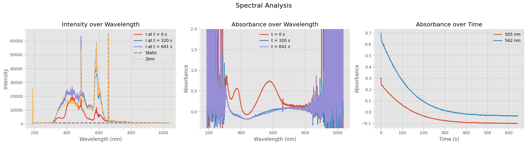
Visualizing Spectral Intensity and Absorbance

This figure provides a comprehensive view of the actinometry data:

1. Left Panel: Raw intensity spectra at three time points, along with the static and zero references.

2. Middle Panel: Corresponding absorbance spectra at the same time points, showing how absorption evolves over time.

3. Right Panel: Absorbance at two key wavelengths (505 nm and 562 nm) plotted as a function of time, highlighting dynamic changes in the sample.

These plots help assess the stability and dynamics of the measured signals and the quality of the zero/static references.

Show code cell source Hide code cell source

import matplotlib.pyplot as plt
import matplotlib.cm as cm

# Use a clean, readable plotting style
plt.style.use("ggplot")

# Set up a figure with 3 subplots side by side
fig, axs = plt.subplots(1, 3, figsize=(18, 5))
fig.suptitle("Spectral Analysis", fontsize=16)

# === Plot 1: Raw Intensities ===
# Show intensity at beginning, middle, and end of acquisition
axs[0].plot(wavelengths, intensities[0, :], label=f"I at t = {timestamps[0]:.0f} s", linewidth=2)
axs[0].plot(wavelengths, intensities[len(intensities)//2, :], label=f"I at t = {timestamps[len(intensities)//2]:.0f} s", linewidth=2)
axs[0].plot(wavelengths, intensities[-1, :], label=f"I at t = {timestamps[-1]:.0f} s", linewidth=2)

# Add static and zero reference spectra for comparison
axs[0].plot(wavelengths, static, '--', label="Static", linewidth=2)
axs[0].plot(wavelengths, zero, '--', label="Zero", linewidth=2)

axs[0].set_title("Intensity over Wavelength")
axs[0].set_xlabel("Wavelength (nm)")
axs[0].set_ylabel("Intensity")
axs[0].legend()

# Add major and minor grid for clarity
axs[0].grid(True, which='major', linestyle='--', linewidth=0.6, color='gray', alpha=0.5, zorder=0)
axs[0].minorticks_on()
axs[0].grid(True, which='minor', linestyle=':', linewidth=0.3, color='lightgray', alpha=0.4, zorder=0)

# === Plot 2: Absorbance Spectra ===
# Show absorbance at beginning, middle, and end of acquisition
axs[1].plot(wavelengths, absorbance[0, :], label=f"t = {timestamps[0]:.0f} s", linewidth=2)
axs[1].plot(wavelengths, absorbance[len(absorbance)//2, :], label=f"t = {timestamps[len(absorbance)//2]:.0f} s", linewidth=2)
axs[1].plot(wavelengths, absorbance[-1, :], label=f"t = {timestamps[-1]:.0f} s", linewidth=2)

axs[1].set_title("Absorbance over Wavelength")
axs[1].set_xlabel("Wavelength (nm)")
axs[1].set_ylabel("Absorbance")
axs[1].set_ylim(-0.4, 2)
axs[1].legend()

# Grid setup
axs[1].grid(True, which='major', linestyle='--', linewidth=0.6, color='gray', alpha=0.5, zorder=0)
axs[1].minorticks_on()
axs[1].grid(True, which='minor', linestyle=':', linewidth=0.3, color='lightgray', alpha=0.4, zorder=0)

# === Plot 3: Absorbance vs Time at Key Wavelengths ===
# Choose wavelengths of interest (e.g. peaks)
WL = [505, 562]
idxs = [np.argmin(np.abs(wavelengths - wl)) for wl in WL]  # Find closest actual wavelength index

# Plot absorbance vs time for selected wavelengths
for i, idx in enumerate(idxs):
    axs[2].plot(timestamps, absorbance[:, idx], label=f"{wavelengths[idx]:.0f} nm", linewidth=2)

axs[2].set_title("Absorbance over Time")
axs[2].set_xlabel("Time (s)")
axs[2].set_ylabel("Absorbance")
axs[2].legend()

# Grid setup
axs[2].grid(True, which='major', linestyle='--', linewidth=0.6, color='gray', alpha=0.5, zorder=0)
axs[2].minorticks_on()
axs[2].grid(True, which='minor', linestyle=':', linewidth=0.3, color='lightgray', alpha=0.4, zorder=0)

# Adjust layout to prevent overlap
plt.tight_layout(rect=[0, 0, 1, 0.95])
plt.show()

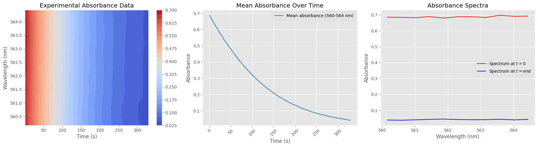
Data Cleaning and Absorbance Subset Preparation

This cell prepares the dataset for focused analysis by:

• Selecting a narrow wavelength range (e.g. 560–565 nm)

• Normalizing absorbance values

• Removing unwanted time points (first spectrum and last 300)

The resulting cleaned subset is suitable for targeted visualization or kinetic analysis.

# === USER PARAMETERS ===
wavelength_range = [560, 565]  # Wavelength range of interest (nm)
remove_first = True            # Whether to remove the first time point
remove_last_n = 300            # Number of last time points to remove
time_filter_indices = [0] + list(range(-300, 0))

# === Select wavelength index range ===
idx_range = np.argmin(np.abs(wavelengths[:, None] - wavelength_range), axis=0)

# Extract absorbance data in selected range
absorbance_subset = absorbance[:, idx_range[0]:idx_range[1]]
absorbance_subset -= np.min(absorbance_subset)  # Normalize (set min to 0)

# Corresponding wavelengths
wavelengths_subset = wavelengths[idx_range[0]:idx_range[1]]

# === Filter time points ===
# Build index list for rows to remove

# Apply filtering
absorbance_subset = np.delete(absorbance_subset, time_filter_indices, axis=0)
timestamps_filtered = np.delete(timestamps, time_filter_indices)



# --- Create 3 plots ---
fig, axs = plt.subplots(1, 3, figsize=(18, 5))

# === 1. Heatmap of absorbance over time and wavelength ===
X, Y = np.meshgrid(timestamps_filtered, wavelengths_subset)  # Create grids for contour plot
contour = axs[0].contourf(X, Y, absorbance_subset.T, levels=30, cmap="coolwarm")
axs[0].set_title("Experimental Absorbance Data")
axs[0].set_xlabel("Time (s)")
axs[0].set_ylabel("Wavelength (nm)")
fig.colorbar(contour, ax=axs[0])  # Add colorbar to show absorbance scale

# === 2. Mean absorbance over time ===
mean_absorbance = np.mean(absorbance_subset, axis=1)
axs[1].plot(timestamps_filtered, mean_absorbance,
            label=f"Mean absorbance ({wavelengths_subset[0]:.0f}-{wavelengths_subset[-1]:.0f} nm)",
            color='tab:blue')
axs[1].set_title("Mean Absorbance Over Time")
axs[1].set_xlabel("Time (s)")
axs[1].set_ylabel("Absorbance")
axs[1].tick_params(axis="x", rotation=45)
axs[1].legend()
axs[1].grid(True)

# === 3. Compare start and end absorbance spectra ===
axs[2].plot(wavelengths_subset, absorbance_subset[0, :], label="Spectrum at $t=0$", color='red')
axs[2].plot(wavelengths_subset, absorbance_subset[-1, :], label="Spectrum at $t=end$", color='blue')
axs[2].set_title("Absorbance Spectra")
axs[2].set_xlabel("Wavelength (nm)")
axs[2].set_ylabel("Absorbance")
axs[2].legend()
axs[2].grid(True)

# Improve layout spacing
plt.tight_layout()
plt.show()

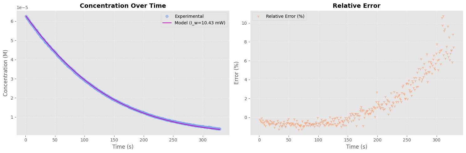
Kinetic Modeling and LED Power Estimation

This section fits the photokinetics model to the experimental concentration curve derived from absorbance data, to estimate the effective LED power.

• Assumes first-order photon absorption

• Uses scipy.integrate.solve_ivp for integration

• Fits using curve_fit with LED power as a free parameter

# === USER PARAMETERS ===
wl = 505  # nm (LED wavelength)
volume = 14e-4  # L
l = 1  # cm (optical path length)
eps_closed_505 = 0.6e4  # M^-1.cm^-1
eps_closed_562 = 1.1e4  # M^-1.cm^-1
I_w_initial_guess = 14.27e-3  # Initial guess (W)
QY_CF2OF = np.power(10, -2.67 + 526 / wl)  # Quantum yield estimation from literature

print(f"Quantum Yield (QY_CF2OF): {QY_CF2OF:.4f}")

from scipy.integrate import solve_ivp
from scipy.optimize import curve_fit

# === Physics constants ===
h = 6.62607004e-34  # Planck constant (J.s)
NA = 6.02214086e23  # Avogadro number (mol^-1)
c_vacuum = 299792458  # m/s
v = c_vacuum / (wl * 1e-9)  # Frequency (Hz)

# === Experimental concentration from absorbance ===
C_exp = mean_absorbance / (eps_closed_562 * l)
C0 = C_exp[0]

# === ODE definition ===
def dC_dt(t, C_closed, I_w):
    I_0 = I_w / (h * v * NA) / volume  # Photon flux [mol photons / L]
    I_abs = I_0 * (1 - np.exp(-eps_closed_505 * C_closed * l * np.log(10)))
    return -QY_CF2OF * I_abs

# === Fitting function wrapper ===
def model(t, I_w, offset):
    sol = solve_ivp(dC_dt, [t[0], t[-1]], [C0], t_eval=t, args=(I_w,))
    if not sol.success:
        print("⚠️ ODE solver failed:", sol.message)
        return np.full_like(t, np.nan)
    return sol.y[0] + offset

# === Fit parameters ===
initial_guess = (I_w_initial_guess, 0)
bounds = ([0, -1], [100e-3, 1])  # Bounds for I_w and offset

print("=== Starting curve fit ===")
popt, pcov = curve_fit(model, timestamps_filtered, C_exp, p0=initial_guess, bounds=bounds)
uncertainties = np.sqrt(np.diag(pcov))

# === Report fitted parameters ===
print("\n=== Fit Results ===")
params = ["I_w (W)", "Offset (M)"]
for name, val, err in zip(params, popt, uncertainties):
    print(f"{name}: {val:.6f} ± {err:.6f}")

# === Compute fitted curve ===
fitted_values = model(timestamps_filtered, *popt)

# === Plotting ===
fig, axs = plt.subplots(1, 2, figsize=(15, 5))
colors = ["#81a3e8", "#f9955e", "m"]

# Plot: Concentration vs Time
axs[0].plot(timestamps_filtered, C_exp, "o", color=colors[0], label="Experimental", alpha=0.6)
axs[0].plot(timestamps_filtered, fitted_values, "-", color=colors[2], label=f"Model (I_w={popt[0]*1e3:.2f} mW)")
axs[0].set_title("Concentration Over Time", fontsize=14, fontweight="bold")
axs[0].set_xlabel("Time (s)")
axs[0].set_ylabel("Concentration (M)")
axs[0].grid(True, linestyle="--", alpha=0.5)
axs[0].legend()

# Plot: Relative Error
relative_error = (C_exp - fitted_values) * 100 / C_exp
axs[1].plot(timestamps_filtered, relative_error, "1", color=colors[1], label="Relative Error (%)", alpha=0.8)
axs[1].set_title("Relative Error", fontsize=14, fontweight="bold")
axs[1].set_xlabel("Time (s)")
axs[1].set_ylabel("Error (%)")
axs[1].grid(True, linestyle="--", alpha=0.5)
axs[1].legend()

plt.tight_layout()
plt.show()

Quantum Yield (QY_CF2OF): 0.0235
=== Starting curve fit ===

=== Fit Results ===
I_w (W): 0.010431 ± 0.000024
Offset (M): 0.000000 ± 0.000000