Examples#

Here are a few examples:

Generate and visualize a vascular network#

In this example, we will demonstrate how to generate and visualize a vascular network from OxyGenie.pgvnet.

Imports and Setup

First, we import the necessary libraries, including OxyGenie.pgvnet, NumPy, and Matplotlib for visualization.
```
import OxyGenie.pgvnet as pgv
import numpy as np
import matplotlib.pyplot as plt
from matplotlib.colors import LinearSegmentedColormap
plt.style.use("bmh")
```
- OxyGenie.pgvnet: The module used for creating vascular networks.
- LinearSegmentedColormap: Creates custom color maps for visualization.

Custom Color Map Definition

We define a custom color map to visualize the network with a smooth gradient.

# Define the colors
colors = ["white", "#4B0082", "#E6BEFF"]
# Create a colormap with linear transitions
custom_cmap_lavande = LinearSegmentedColormap.from_list(
    "custom_cmap", colors, N=256)

LinearSegmentedColormap: Defines a color gradient transitioning from white to lavender.

Global Parameters Setup

Next, we define several global parameters that control the behavior of the vascular network generation.
```
# Global parameters
Lc = 30         # Average segment length
lrang = 10      # Length variation
grid_size = 1000  # Grid size
alpha = np.pi / 4  # Angle variation amplitude
start_x, start_y = grid_size // 2, grid_size - 10  # Bottom-center starting point
initial_angle = 0
```
- Lc: Average segment length of branches in the network.
- lrang: Variation in segment lengths.
- grid_size: Size of the grid (1000x1000 pixels).
- alpha: Angle variation amplitude for branch angles.
- start_x, start_y: Starting point for branch generation.
- initial_angle: Starting angle for the first branch.
Grid Initialization

A grid is initialized to hold the vascular network. The grid size is set to grid_size and is filled with zeros.
```
# Initialize the grid
grid = np.zeros((grid_size, grid_size), dtype=np.uint8)
```
- grid: Represents the space where the vascular network will be generated.

Pipeline Setup

The PGPipeline is set up with a series of operations that define how branches and the network are generated.

# Create the sequence of operations
sequence = pgv.PGPipeline([
    pgv.BranchGen((Lc, lrang), (initial_angle, alpha / 5), 1),
    pgv.DilationN(3),
    pgv.BranchGen((Lc, lrang), (2 * np.pi, alpha / 3), 4),
    pgv.DilationN(1),
    pgv.BranchGen((Lc, lrang), (2 * np.pi, alpha / 3), 8),
    pgv.DilationN(1),
    pgv.BranchGen((Lc, lrang), (2 * np.pi, alpha / 2), 8),
    pgv.DilationN(1),
    pgv.PGVNet(5),
])

PGPipeline: A pipeline of operations that define how the vascular network will be generated.
BranchGen: Generates branches based on length and angle range.
DilationN: Expands the network after branching.
PGVNet: Final operation that generates the vascular network.

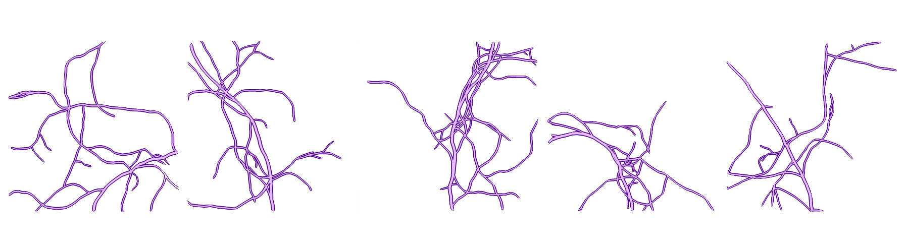
Grid Simulation and Visualization

The pipeline is executed multiple times to generate different variations of the vascular network. We then display the results using Matplotlib.

# Generate n different images
n = 5
fig, axes = plt.subplots(1, n, figsize=(25, 5))

for i in range(n):
    np.random.seed(i)  # Change the random seed for each image
    # Initialize with an empty branch list
    ngrid, nbranchs = sequence(grid.copy(), [(start_x, start_y)])
    ax = axes[i]
    ax.imshow(ngrid, cmap="Purples")
    ax.xaxis.set_visible(False)  # Hide x-axis
    ax.yaxis.set_visible(False)  # Hide y-axis
    ax.set_title(f"Gen n°{i+1}")  # Title showing generation number

plt.tight_layout()
plt.show()

np.random.seed(i): Changes the seed for each generated image to ensure unique results.
sequence(grid.copy(), [(start_x, start_y)]): Executes the pipeline and generates a new vascular network.

Code

Result

Generate and Simulate Tissue Oxygenation#

In this example, we will demonstrate how to generate a vascular network using OxyGenie.pgvnet, and simulate tissue oxygenation based on that network using OxyGenie.diffusion. The process involves generating the vascular network, setting simulation parameters, and visualizing the results.

Imports and Setup

First, we import the necessary libraries, including OxyGenie.pgvnet, OxyGenie.diffusion, NumPy, and Matplotlib for visualization.
```
from OxyGenie.diffusion import *
import OxyGenie.pgvnet as pgv
import matplotlib.pyplot as plt
import numpy as np
plt.style.use("bmh")
```
- OxyGenie.pgvnet: The module used for creating vascular networks.
- OxyGenie.diffusion: Contains methods and function for simulating oxygen diffusion in tissue.
Define Simulation Parameters

We define the parameters required for the diffusion simulation, such as diffusion coefficient, simulation grid size, and time steps.
```
# Simulation parameters
params = {
    "D": 1e-5, "k": 8, "Lx": 0.05, "Ly": 0.05, "T": 0.5, "nt": 2500, "nx": 256 * 2, "ny": 256 * 2,
    "initial_concentration": 100.0, "speed": 1, "step": 10,
}

# Initialize simulation parameters
simparams = SimulationParams(**params)
```
- D: Diffusion coefficient (m²/s).
- k: Absorption coefficient.
- Lx, Ly: Length of the simulation domain in x and y directions.
- T: Total time of simulation.
- nt: Number of time steps.
- nx, ny: Grid resolution in x and y directions.
- initial_concentration: Initial oxygen concentration.
- speed: Speed of simulation.
- step: Step size for the simulation.
Generate Vascular Network

Next, we generate the vascular network using OxyGenie.pgvnet’s simple_generation method, which simulates a basic network of vessels.
```
# Generate vascular network
Vnet = pgv.simple_generation(grid_size=1280)
```
- Vnet: A generated vascular network stored as an array.
Run Diffusion Simulation

With the network generated, we simulate oxygen diffusion using OxyGenie.diffusion.run_simulation. The simulation is run on the generated vascular network, with the oxygen concentration modeled over time.
```
# Run simulation with generated vascular network
L_result = run_simulation(simparams, FromPGVNet(Vnet[0]), C_0_cst=True)
```
- L_result: The result of the simulation containing oxygen concentration values over time.

Custom Simulation Example

You can also run the simulation with a custom initial concentration and diffusion parameters. This demonstrates flexibility in defining the initial conditions for the simulation.

# Custom simulation parameters
C = np.zeros((simparams.nx, simparams.ny))
C[120:130, 120:130] = 1

X, Y = np.meshgrid(np.linspace(-1, 1, simparams.ny), np.linspace(-1, 1, simparams.nx))
D = np.exp(-((X)**2 + (Y-1)**2) / 1.5)

k = np.ones((simparams.nx, simparams.ny))

# Run custom simulation
L_result = run_simulation(simparams, FromCustom(C, D, k), C_0_cst=True)

C: Custom initial concentration array.
D: Custom diffusion coefficient array.
k: Custom absorption coefficient array.

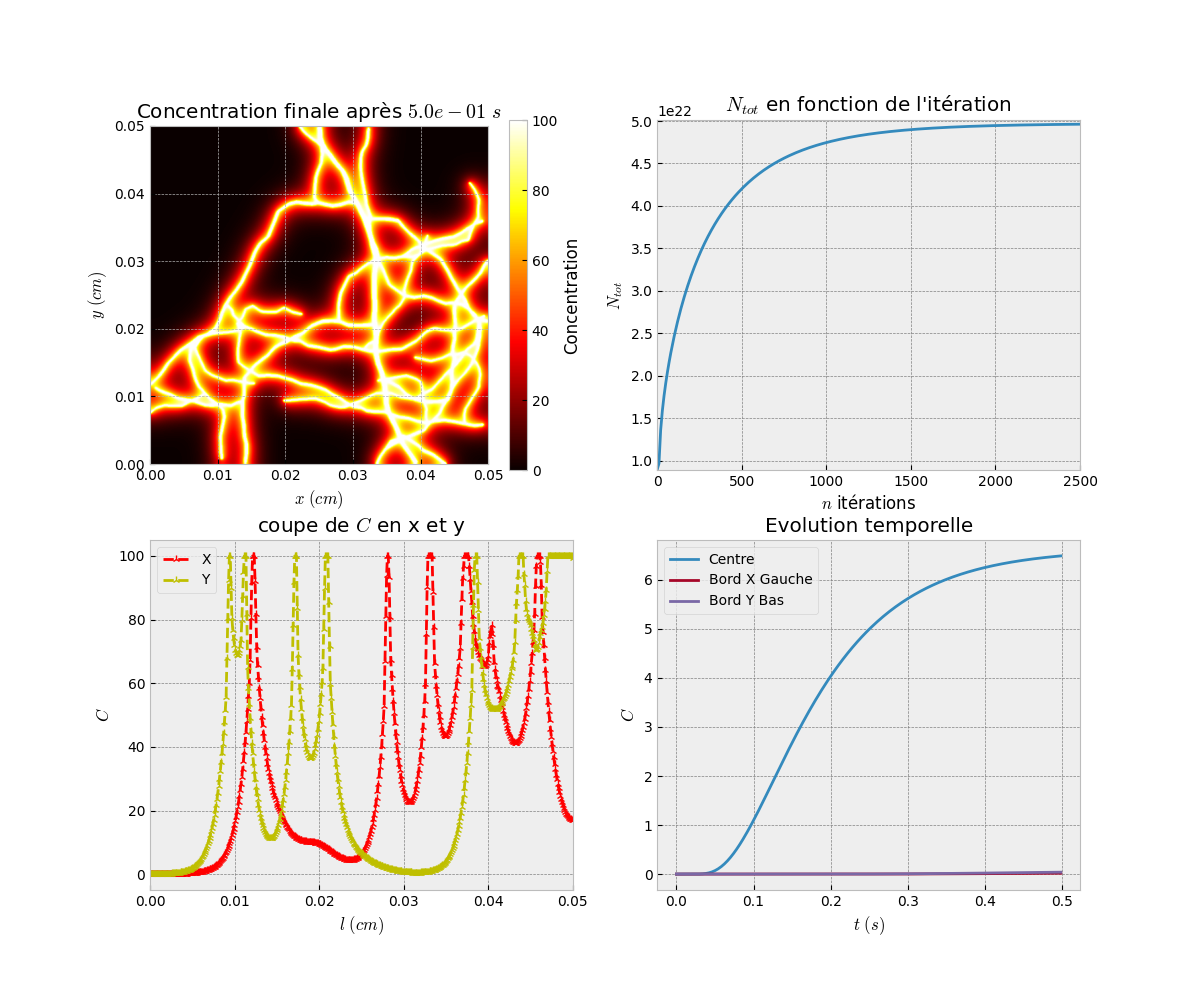
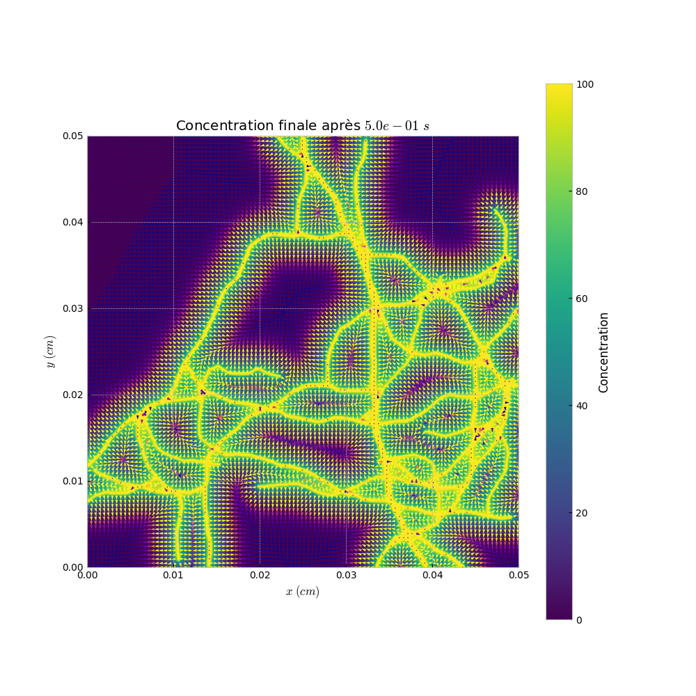
Visualization

Finally, we visualize the results of the simulation. We display the concentration at the final time step and generate animations of the diffusion process.
```
# Visualization of the results
Simu_plot.simple(simparams, L_result[-1], simparams.D_mat)
Simu_plot.anim(simparams, L_result, anim=True)
Simu_plot.anim_vect(simparams, L_result, s_ech=5)
```
- Simu_plot.simple: Displays the concentration at the final time step.
- Simu_plot.anim: Creates an animation of the diffusion process.
- Simu_plot.anim_vect: Generates an animation with vector representation.

Code

Result

Generate and Simulate Oxygen Diffusion with Neural Network#

In this example, we will demonstrate how to generate a vascular network using OxyGenie.pgvnet, simulate tissue oxygenation using OxyGenie.diffusion, and enhance the simulation with a trained neural network model, EUNet, from OxyGenie.learn.

Imports and Setup

We begin by importing the necessary libraries, including OxyGenie.diffusion, OxyGenie.pgvnet, OxyGenie.learn.EUNet, NumPy, Matplotlib, and Torch for handling the neural network.
```
import numpy as np
import torch
import matplotlib.pyplot as plt
from tqdm import tqdm
import OxyGenie.diffusion as simu
import OxyGenie.pgvnet as pgv
from OxyGenie.learn import EUNet
```
- EUNet: A pre-trained neural network for oxygen diffusion predictions.
- OxyGenie.pgvnet: The module for generating vascular networks.
- OxyGenie.diffusion: Contains methods for simulating oxygen diffusion.
- torch: Used for loading the pre-trained model and running inference.
Load the Pre-trained Neural Network

We load the pre-trained model weights into EUNet using the torch.load method.
```
# Load the pre-trained model weights
model = EUNet()
model.load_state_dict(torch.load("model2_weights_6E.pth"))
```
- EUNet: The model is used for predicting oxygen concentrations based on the vascular network.

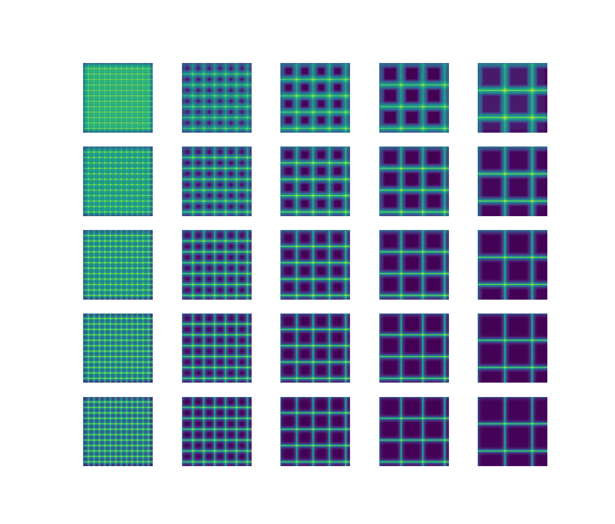
Simulation with Varying Parameters

We simulate the diffusion process on a grid, using the pre-trained model to predict outcomes for varying input parameters.

n = 5
lk = np.linspace(1, 10, n)
fig, ax = plt.subplots(n, n, figsize=(12, 12))

for j in tqdm(range(n)):
    mat = np.zeros((512, 512))
    step = 40 * (j + 1)
    mat[:, ::step] = 255
    mat[::step, :] = 255

    for i in range(n):
        params = [float(lk[i]), 5e-3]
        out = model.predict(mat.astype(np.float32), params)
        ax[i, j].imshow(out, vmin=0, vmax=120)
        ax[i, j].axis("off")
plt.show()

mat: A matrix representing the grid with different spacing (steps).
params: The parameters used to adjust the simulation based on the neural network prediction.
model.predict: The pre-trained model generates predictions based on the input matrix.

Simulating Oxygen Diffusion with Random Network

We generate a random vascular network and simulate oxygen diffusion. The results from the model are used as the initial conditions for the simulation.

np.random.seed(5)
k_random = 1

T_simu_rp = -2 / 9 * k_random + 2.5 - 2 / 9
nt_efficient = int(T_simu_rp * 5000)

params = {
    "D": 1e-5, "k": k_random, "Lx": 0.05, "Ly": 0.05, "T": 0.25, "nt": 2500, "nx": 256 * 2, "ny": 256 * 2,
    "initial_concentration": 100.0, "speed": 1, "step": 10,
}
simuparams = simu.SimulationParams(**params)

# Generate random vascular network
V_net = pgv.simple_generation(grid_size=1280)[0]

sp = pgv.sp_ratio(V_net)

# Prepare input for the model
X_1 = V_net.copy()
X_2 = [float(k_random), float(sp)]

# Run prediction using the neural network
out = model.predict(V_net.astype(np.float32), X_2)
out[out > 100] = 100

# Simulate oxygen diffusion with the predicted initial conditions
L_result = simu.run_simulation(simuparams, simu.FromPGVNet(V_net), C_0_cst=True, save_last_only=False, C0=out)

Y = L_result[-1]  # Final simulation result

k_random: Random value chosen for the absorption coefficient.
V_net: The generated vascular network.
model.predict: The model’s prediction is used as the initial concentration for the diffusion simulation.
L_result: The results of the diffusion simulation.

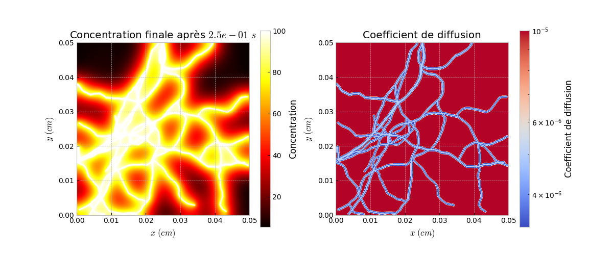
Visualization of the Simulation Results

We visualize the results of the diffusion simulation by displaying the concentration at the final time step and generating animations of the diffusion process.
```
f, a = plt.subplots(1, 2)
a[0].imshow(L_result[len(L_result)//2], cmap="hot")
a[1].imshow(Y, cmap="hot")
a[1].axis("off")
a[0].axis("off")
plt.show()

simu.Simu_plot.simple(simuparams, L_result[-1], simuparams.D_mat)
simu.Simu_plot.anim(simuparams, L_result)
```
- L_result[len(L_result)//2]: Displays the intermediate result of the simulation.
- Y: Displays the final result of the simulation at the steady state.
- Simu_plot.simple: Visualizes the final concentration.
- Simu_plot.anim: Creates an animation of the simulation process.

Code

Result